9 February 2023 | Blog

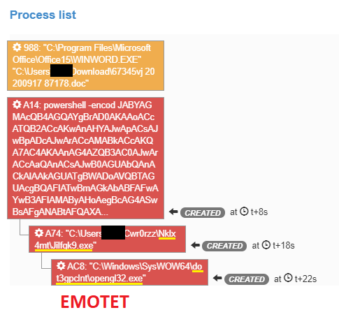
In many of the security incidents we deal with, we see random strings in the artifacts. This can be process names, access paths, registry keys, etc. Random values are found in many data sources and are often associated with malicious activity. This mission is carried out by our Use Case Factory, our unit specialized in content production and continuous improvement.

Figure 1: Process Tree – dropper Emotet | Source: Sandbox Orange Cyberdefense P2A
In our CyberSOCs, it’s essential to identify these values automatically through our detection tools. The objective is to build scenarios around these anomalies and detect threats in a constrained environment: our SIEMs. To do this, we need to develop a mechanism that has the least possible impact on their performance while providing convincing results.
In this post, we present the research we’ve done to distinguish a random value, the method we applied to build a detection function, and finally, the implementation in our SIEMs, illustrated by a use case.
With a simple search using the internet, we can find many GitHub projects, which cover this need. Even if they seem interesting, we have chosen not to use them for several reasons:
So we think it makes more sense to develop our own tool. For this, we will use a dataset from our research environment. These datasets contain more than 600 entries, mostly process names but also some file names. It also has about 50 manually identified random characters.

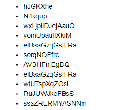
Figure 2: Random process name list related to malware | Source: Orange Cyberdefense CyberSOC
We can notice a strong recurrence of unusual letters such as W or Z. Also, we see amazing bigrams such as WX or XK. This is not visible in the example above, but we can notice a more critical use of non-alpha characters and capital letters’ essential use. Letter frequency analysis is a technique used in cryptanalysis to decode messages encrypted by character substitution (Caesar encryption). It’s based on the premise that in everyday language, some letters are used more than others.
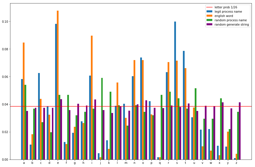
The graph below illustrates the frequency of use of letters in common words, legitimate process names, put into perspective with random values.

Figure 3: Letter frequency graph | Source: Orange Cyberdefense CyberSOC
We can see that the frequencies are much more homogeneous for random chains. Conversely, the distribution is very different for non-random chains. Some characters are used a lot, and others very little. The presence of rare letters such as q or z can be used as a marker.
If this feature is interesting, it’s not enough. However, it’s necessary to associate other markers to ensure that a word is random. For this, we can use the bigram (sequence of 2 letters). This study shows that certain bigrams (JQ, QG, QK, QY, QZ, WQ, and WZ) do not appear in English words. Conversely, some bigrams such as TH or HE are very common. Therefore, it can also be used as a marker. For this, we will use TF-IDF (Term Frequency – Inverse Document Frequency). We will, however, adapt the calculation to increase the point of rare values.
Using the legitimate process names coupled with a random list of English language words, we create two matrices: one for letters and one for bigrams. They will then be used to score a string. The higher the score, the more random the word is.
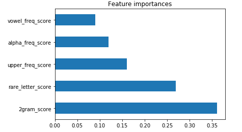
Our research studied other characteristics such as vowel frequency, the ratio of upper case, lower case characters, and the ratio of alpha, non-alpha characters. Using a supervised learning algorithm based on decision trees, we identify the most determining characteristics.

Figure 4: features importance to determining the randomness of a word | Source: Orange Cyberdefense CyberSOC
As shown in this graph, 2grams and rare letters are the two most critical characteristics for identifying a random string. We will keep only these two and add upper_freq as weighting.
Now that we have identified the variables to discriminate a random string and a detection method, we can build a prototype. Based on the results obtained during the previous analyses, thresholds are configured, and the function is applied to our dataset. Finally, we compare the results obtained by our prototype with the labels that we have associated with each value. Our dataset contains two titles: BAD for the random chains, LEGIT for the others. Our prototype also returns a SUSPICIOUS category for chains that are difficult to classify.
The result is rather satisfactory; the dataset contains 403 strings, of which 45 are random. Thirty-six of them have been correctly identified, and a large part of the non-random strings have been correctly detected. Only 8 false positives and 4 false negatives were detected.
If we take a look at errors, we see :
Errors can be reduced in different ways:
As the dataset was a little small, the prototype was also tested on an artificial dataset. Overall, if there were some errors, the results are rather good (more than 90% true positive and false negative). The prototype can, therefore, be considered functional.
The next step is to integrate this mechanism into our SIEMs. So the prototype is ported in a Splunk® app. The impact on performance is anecdotal. The SIEM version also incorporates new features such as returning a score instead of a class. It also allows for generating a scoring matrix for the different parts. This makes it possible to directly set up another scoring mechanism in SIEM or feed a machine learning algorithm.
The application is used to develop new detection mechanisms. In the example below, we try to identify processes with a random name. As previously mentioned, we can integrate the process’s prevalence (i.e., the number of machines on which it is running) into our scoring mechanism. This allows us to reduce the false positive rate with a lower scoring matrix. Note also that we can couple this mechanism with a whitelist.

Figure 6: Example result obtained on Splunk® lab | Source: Orange Cyberdefense CyberSOC
The result shows that the command does allow to identify processes with a random name and, in our case, to detect a threat.
This case is a good illustration of the need always to evolve these detection tools. From this simple application, many new scenarios can be set up. Random processes are just one example among many (registry keys, file names, URL, etc.). A random name is not systematically linked to a threat. On the other hand, using this mechanism and other indicators such as Threat Intelligence or prevalence can enrich detection.

In our CyberSOCs, it’s essential to identify these values automatically through our detection tools. The objective is to build scenarios around these anomalies and detect threats in a constrained environment: our SIEMs. To do this, we need to develop a mechanism that has the least possible impact on their performance while providing convincing results.
In this post, we present the research we’ve done to distinguish a random value, the method we applied to build a detection function, and finally, the implementation in our SIEMs, illustrated by a use case.

With a simple search using the internet, we can find many GitHub projects, which cover this need. Even if they seem interesting, we have chosen not to use them for several reasons:
So we think it makes more sense to develop our own tool. For this, we will use a dataset from our research environment. These datasets contain more than 600 entries, mostly process names but also some file names. It also has about 50 manually identified random characters.

We can notice a strong recurrence of unusual letters such as W or Z. Also, we see amazing bigrams such as WX or XK. This is not visible in the example above, but we can notice a more critical use of non-alpha characters and capital letters’ essential use. Letter frequency analysis is a technique used in cryptanalysis to decode messages encrypted by character substitution (Caesar encryption). It’s based on the premise that in everyday language, some letters are used more than others.
The graph below illustrates the frequency of use of letters in common words, legitimate process names, put into perspective with random values.

We can see that the frequencies are much more homogeneous for random chains. Conversely, the distribution is very different for non-random chains. Some characters are used a lot, and others very little. The presence of rare letters such as q or z can be used as a marker.
If this feature is interesting, it’s not enough. However, it’s necessary to associate other markers to ensure that a word is random. For this, we can use the bigram (sequence of 2 letters). This study shows that certain bigrams (JQ, QG, QK, QY, QZ, WQ, and WZ) do not appear in English words. Conversely, some bigrams such as TH or HE are very common. Therefore, it can also be used as a marker. For this, we will use TF-IDF (Term Frequency – Inverse Document Frequency). We will, however, adapt the calculation to increase the point of rare values.
Using the legitimate process names coupled with a random list of English language words, we create two matrices: one for letters and one for bigrams. They will then be used to score a string. The higher the score, the more random the word is.
Our research studied other characteristics such as vowel frequency, the ratio of upper case, lower case characters, and the ratio of alpha, non-alpha characters. Using a supervised learning algorithm based on decision trees, we identify the most determining characteristics.
As shown in this graph, 2grams and rare letters are the two most critical characteristics for identifying a random string. We will keep only these two and add upper_freq as weighting.
Now that we have identified the variables to discriminate a random string and a detection method, we can build a prototype. Based on the results obtained during the previous analyses, thresholds are configured, and the function is applied to our dataset. Finally, we compare the results obtained by our prototype with the labels that we have associated with each value. Our dataset contains two titles: BAD for the random chains, LEGIT for the others. Our prototype also returns a SUSPICIOUS category for chains that are difficult to classify.
The result is rather satisfactory; the dataset contains 403 strings, of which 45 are random. Thirty-six of them have been correctly identified, and a large part of the non-random strings have been correctly detected. Only 8 false positives and 4 false negatives were detected.
If we take a look at errors, we see :
Errors can be reduced in different ways:
As the dataset was a little small, the prototype was also tested on an artificial dataset. Overall, if there were some errors, the results are rather good (more than 90% true positive and false negative). The prototype can, therefore, be considered functional.

The next step is to integrate this mechanism into our SIEMs. So the prototype is ported in a Splunk® app. The impact on performance is anecdotal. The SIEM version also incorporates new features such as returning a score instead of a class. It also allows for generating a scoring matrix for the different parts. This makes it possible to directly set up another scoring mechanism in SIEM or feed a machine learning algorithm.
The application is used to develop new detection mechanisms. In the example below, we try to identify processes with a random name. As previously mentioned, we can integrate the process’s prevalence (i.e., the number of machines on which it is running) into our scoring mechanism. This allows us to reduce the false positive rate with a lower scoring matrix. Note also that we can couple this mechanism with a whitelist.
The result shows that the command does allow to identify processes with a random name and, in our case, to detect a threat.
This case is a good illustration of the need always to evolve these detection tools. From this simple application, many new scenarios can be set up. Random processes are just one example among many (registry keys, file names, URL, etc.). A random name is not systematically linked to a threat. On the other hand, using this mechanism and other indicators such as Threat Intelligence or prevalence can enrich detection.